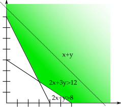
Fig:graphSolutionEx An example for a graphical solution of an LP. The optimal solution is (3,2)
Recall from the introduction that a linear program is defined by a linear objective function and a set of constraints for . For reasons that will become clear in a few paragraphs (and even clearer in the next part of this series), I will write the variables as a column vector , where I use the superscript to indicate transposition so that I can write column vectors in the rows of this text.
When we treat the variables as a vector like this, it makes sense to call the number of variables the dimension of the LP. I will call vectors that satisfy all constraints feasible. If there is no such vector, the problem is infeasible.
Solving 1-dimensional LPs is trivial. We have just one variable . The cost function either becomes bigger as increases or smaller, so we immediately know whether we’re looking for the biggest that satisfies the constraints or the smallest. The set of feasible is then the intersection of the rays defined be the constraints. For example
The constant before the in the cost function is positive, so in order to minimize the objective value we need to minimize . The constraints can be simplified to and thus the optimal value is .
In two dimensions we can use a very similar strategy. The cost function still tells us in which direction to move and the intersection of the constraints gives us a feasible region. We use a graphical approach to see the set of feasible values for .
If you write an equals sign like this , you get an equation for a line. If you write the constants as a vector , you can write the line equation using the dot product: . Note that is orthogonal to the line. Why is that so? Take some that lies on the line, i.e. it solves the above equation. Moving by some amount along the line (this means is a vector parallel to the line) results in another vector that lies on the line and hence still satisfies the equation. The dot product is distributive so we can write . We know (since this is how we chose ), so the second summand must be zero. When the dot product is zero, the two vectors are orthogonal.
Now consider what happens to the equation when we take an from the line and move it by some that is not parallel to the line. It depends on . If the dot product is positive, the left hand side becomes too big for the equality, otherwise it becomes too small. The dot product is positive if points somewhat in the same direction as (more formally, can be decomposed in two vectors, and , such that is orthogonal to and is for some positive real ).
So if we take the original inequality, it cuts the 2D plane in two parts, left and right from the line. Which part satisfies the inequality depends on the direction of and whether we have a or a . The set of points that satisfy the inequality is called a halfplane.
The feasible region of the problem, i.e. all the points that satisfy all constraints, is then the intersection of all the halfplanes.
The cost function also defines a line, or rather, a family of lines, one for each objective value, namely the solutions for for each objective value . If the intersection of this line with the feasible region is not empty, there is a solution (any point in the intersection) with cost . The cost vector is orthogonal to the line defined by . The goal is to shift the line as far in negative direction as possible without leaving the feasible region. Take for example the following LP

Fig:graphSolutionEx An example for a graphical solution of an LP. The optimal solution is (3,2)
The cost vector is and the two constraints define two half-planes. For every value of the cost function, we have a line . See figure [Fig:graphSolutionEx]. We want to find the smallest value of such that is a feasible solution. So we start with some arbitrary in the feasible region (picking it is the eye-balling step) and then gradually move it in direction (i.e. we subtract small multiples of ). Once we find that we can’t move our solution any further without leaving the feasible region, we have reached the optimum.
A somewhat weaker operation than picking a feasible solution to LP is picking an objective value and finding out whether this objective value can be achieved.
To do so, we can add a new constraint, namely . This constraint adds another half-plane that constrains the feasible region. If this makes the feasible region empty, there is no solution with an objective value at most . If the feasible region still contains more than one point, then we can decrease a little more. We have reached the optimal if the feasible region contains only one point. Now, if we had a method to check whether a feasible region is empty or not, this would give us an algorithm to solve linear programs with many evaluations of the feasibility algorithm.
Now that we know how to solve 1D LPs rigorously and 2D LPs with a graphical method, let us try to find a method that works for arbitrary dimensions. As we already can solve low-dimensional LPs, it makes sense to try and get there via dimensionality reduction.
Fourier-Motzkin elimination is a method to reduce the dimension of an LP by one without changing feasibility. If we keep reducing the dimension one by one, we eventually reach the 1D case, where we can test feasibility easily. The objective value is disregarded by this method, we only care about feasibility. By adding an additional constraint as described above we can transform the optimization problem to a feasibility problem. In an exercise you will show how to reconstruct an optimal solution.
The method works by rearranging the constraints to solve for one variable and then introducing enough new constraints to make the variable unnecessary. As an example we will use this 2D LP.
Exercise: Draw the feasible region for this LP.
We want to eliminate . So first we rearrange all constraints to have just on the left side. We get
Now we can combine the constraints where with the constraints where . As we have two of each, we get four constraints.
Exercise Add these constraints to your picture.
We can simplify to
which further simplifies to
and lastly
If you did the exercise above correctly, you will see that projecting the feasible region down to the axis leaves you with the interval . Note that the simplification we did to the constraints after eliminating was in fact the procedure to eliminate . A 0-dimensional LP has no variables, just a bunch of inequalities involving numbers and the feasibility check is just some calculation.
Exercise: Instead of , eliminate . Does your result match your picture?
In general Fourier-Motzkin elimination works as follows:
Exercise: Use Fourier-Motzkin Elimination to find not just the optimal objective value, but also the optimal solution.
Let’s try to prove that Fourier-Motzkin Elimination is correct, that is, it reduces the dimension by one, without changing satisfiability. Let us first define the projection of a set of vectors. Since we can choose the order of our variables without changing the problem, it suffices to deal with the case where we drop the last coordinate of each vector.
Definition Let be a vector. Then is the projection of on the first coordinates. For a set of vectors , let be the set where we apply on every element.
It is easy to see that for any non-empty set , is also non-empty. So if is the feasible set of our linear program, projecting it down doesn’t change feasibility. So far so good. Unfortunately we don’t have the feasible region given as a point set, it’s given by the inequalities. Hence we need to use Fourier Motzkin elimination instead of just dropping a coordinate. Next we will show that Fourier Motzkin elimination indeed computes the projection.
Proof Let be the feasible region of our LP, and let be the feasible region of the LP after we remove the last variable via Fourier Motzkin Elimination. We show . We do so by proving mutual inclusion, that is and
. That means we have a point in and we want to find a in that corresponds to it. In the vector has another component, so let us write in a slight abuse of notation . We don’t know (and there are in general many that get mapped to ) but we know that it had to satisfy the constraints.
There are three kinds of constraints in our LP after we rearrange the inequalities to have only on the left hand side, as explained above. Type 1 constraints don’t contain and hence have no influence on , so if satisfies them also satisfies them. For type 2 and type 3 inequalities, we know that there is an that satisfies all of them.
We constructed by combining type 2 and type 3 constraints. Let be the r.h.s. of the tightest type 2 constraint, that is, the constraint where the right hand side evaluates to the smallest number when we plug in , and similarly let be the r.h.s. of the tightest type 3 constraint. Note that then is the tightest constraint for that we have in . Since satisfies all constraints, we know and hence . Thus satisfies the constraints for and hence .
. For this direction also we have to choose so that satisfies the constraints for . As in the other direction let be the r.h.s. of the tightest type 2 constraint, and let be the r.h.s. of the tightest type 3 constraint. Then we can simply choose any . This interval can’t be empty, because we have the constraint in our constraint set for and satisfies all of those constraints.
And this concludes our proof.
So with Fourier Motzkin elimination we have a method of checking feasibility for Linear Programs: Eliminate dimensions until no variables remain and do the math to see whether each inequality is satisfied. Together with your method for transforming optimization to repeated feasibility, we can now solve Linear Programming. Unfortunately Fourier Motzkin Elimination gets pretty expensive for large dimensions as you’ll see in the next exercise.
Exercise What’s the runtime of an -step Fourier Motzkin Elimination? Hint: How many constraints do you introduce in each step?
Next part: Polyhedra
Click here to go back to the index